What is the relationship between reinforcement, Q and deep-Q learning?

Formulating Reinforcement Learning

Reinforcement learning (RL) is centered around the principle of action followed by reward. Just like most machine learning algorithms, reinforcement learning is an optimization technique where we maximize reward. Read more about the relationships between the types of Q learning.

• In case of RL, the learning is online, i.e., the model updates and predictions are done in tandem.
• The core principle is to perform an action given a state and assess the reward for the same in order to adjust the strategy for your future actions and states. This is formulated as follows:
• We define the mapping between actions aₜ and states sₜ, i.e. our policy (strategy) π, at a given time t.
• The cumulative discounted reward is defined as...

where rᵢ reward at time i. Essentially, the total reward accumulated up until time t.

• The action-value function is expected value of cumulative reward, i.e.,

This is what we optimize (maximize), i.e., converge to the optimal action-value function

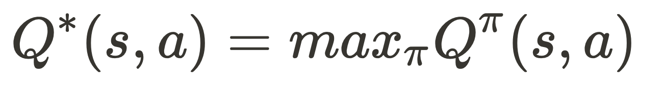
This can be done via Bellman’s equation as follows

where s' the next state and r is the reward for action a on state s.

Q Learning

Q Learning builds upon Bellman’s Equation by introducing stochasticity in the way our agent can perform optimal actions, where optimality hinges on maximizing the reward or more specifically, the action-value. This is defined as follows.

‍

Denoting r as R(s,a), for a probability P(s,a,s') for transitioning to state s', we get

where Q(s,a) is the Q-value (action-value) for action a on state s.

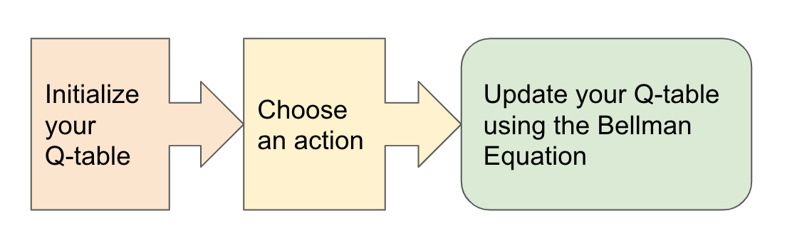
The Learning Process

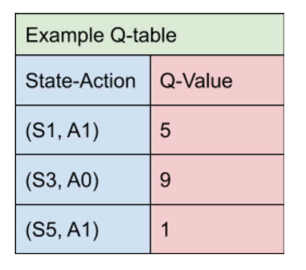
In the RL environment, for a given set of starting states and actions, we want to converge the table state-action Q-values to their corresponding optimal values.

So how do we train the agent to converge Q-values to and maintain an optimal state?

Answer: Use the Temporal Difference (TD).

Referring to the previously defined approximation of Q-value, we can define TD as its difference with the current Q-value. TD represents how far off are we from the ideal or target value compared to an earlier stage.

Given a learning rate ɑ, the q-value updates are done as follows for time t

Inserting the value for TD(a,s) we get

Deep Q Learning

For each learning update in Q Learning, we need to compute Q-values for all states-action pairs. This is practically possible only for a reasonably small set of discrete states. This is because the learning complexity will be primarily determined by size of the state space, i.e., the more states, the longer an update takes. This begs the question…

What happens if there’s just too many states to calculate for?

Answer: Use deep learning to approximate the optimal Q-value`

So we essentially replace the Q-table with a neural network.

Critically, Deep Q-Learning replaces the regular Q-table with a neural network. Rather than mapping a state-action pair to a q-value, a neural network maps input states to (action, Q-value) pairs.

Using the highest Q-value across all actions, we update the neural network weights using mean squared loss over $TD$, thereby iteratively converging towards the optimal Q-values for all states. The loss is defined as follows.

The relationships between the types of Q learning conclusions

Q Learning

Reinforcement learning that

• Iteratively adjusts state-action policy by maintaining a table of state-action pairs and their corresponding reward (Q-value) values and
• Updates these values by evaluating all possible combinations of actions on all states and picking those that produce the cumulatively highest Q-value

Deep Q Learning

RL with the same core principle of Q Learning, but

• Instead of calculating and evaluating all possible state-action pairs and their corresponding Q-value, this method leverages a Deep Neural Network to pass states as input vectors and output Q-values corresponding to all valid actions on the state.
• The optimal Q-value is used to update the network

Deep Q Network

The Deep Convolutional Neural Network used to ingest state as image input (tensors) and output Q-value for all possible actions on the state.

Model Free vs Model Based

RL algorithms can be mainly divided into two categories – model-based and model-free.

Model-based, as it sounds, has an agent trying to understand its environment and creating a model for it based on its interactions with this environment. In such a system, preferences take priority over the consequences of the actions i.e. the greedy agent will always try to perform an action that will get the maximum reward irrespective of what that action may cause.

On the other hand, model-free algorithms seek to learn the consequences of their actions through experience via algorithms such as Policy Gradient, Q-Learning, etc. In other words, such an algorithm will carry out an action multiple times and will adjust the policy (the strategy behind its actions) for optimal rewards, based on the outcomes.

References

• ‍An introduction to Q-Learning: Reinforcement Learning‍
• ‍Deep Q-Learning Tutorial: minDQN‍
• Deep Q-Learning | An Introduction To Deep Reinforcement Learning‍
• Model-Based and Model-Free Reinforcement Learning: Pytennis Case Study - neptune.ai

Devron is a next-generation federated learning and data science platform that enables decentralized analytics. Learn more about our solutions, read more of our knowledge base articles, about our federated learning platform, or schedule a demo with us today.